Whew! It’s already the start of Fall semester! That means I am officially a 2nd year graduate student and have completed one (of five-ish) years of my PhD program! Woo! Along with all the other excitement that comes with my second year of grad school, I have now gotten established in my research projects and will be needing to focus on making significant progress before the end of the academic year where I will present (and be tested) on my research material. So! With that said, hopefully I’ve made some good progress over the summer, right!?

Happily, I can report yes! While my research had a bit of a shaky start at the beginning of the last fall semester, this semester I’ve got lots to do and am excited to do it! If you don’t remember where I left off at the beginning of the summer I encourage you to go catch up on my previous post! 🙂

At the beginning of the summer I left off with my two new research endeavors, ‘observing’ simulated data and my second project having to do with instrumentation. These are what I focused on throughout the summer. Let’s start with the second project:

My second project’s goal is to test how reliable it is to measure a signal outside of an instruments designated range. Say my instrument (like a radio) can measure frequencies (like radio stations) between 50 and 100 MHz. If there was some signal I wanted to measure at 150 MHz, I shouldn’t be able to do it, right? Actually – if you know enough about your instrument, you can! The higher signal may not be measured directly by your instrument, but you can pick up a version of it – an alias. If you know the details of how your instrument works you can take this alias and work backwards to find the original signal. 

My project is essentially picking ranges of frequencies and seeing how well I can read a signal outside of this range. I do this by measuring what’s called the Allan Variance. The Allan Variance is a measure of how stable you measurement is – or how much error is associated with your measurement. If you measure your signal several times and average it, the error associated with the measurement will go down – so will the Allan Variance.

My progress over the summer included writing code to compute this Allan Variance and making plots of it for a small sample of data. Once I knew that was working I could consider which frequency ranges I wanted to cover. I did this by measuring the strength of a signal as I increased it’s frequency in small steps. As the signal got further out of the natural range of my instrument, the strength of the signal went down. You can think of strength of a signal like the clarity and volume of a radio station. If the station sounds fuzzy and is quiet, the signal is not very strong.

I measured the strength until I found the frequency that had a strength about one tenth the magnitude of the strength of my lowest frequency measurement – that told me the maximum limit for my frequency ranges! With that knowledge, I decided on the frequency ranges I wanted and went to order filters! These filters are made up of combinations of inductors and capacitors and are constructed in such a way that they will only allow a specific range of frequencies through. By using the filters I know that when I measure the Allan Variance, it is only specific to the range of frequencies for the filter I used.

Looking for and buying these filters was an adventure. I never thought I’d be looking searching for electrical components on a website that specializes in industrial instrumentation equipment. Even so – I did it! and three lovely filters were delivered to my building and are waiting for me – maybe I should name them….

On to the first project! With all of the challenges I encountered in the first 9 months of working on this project, I was beginning to get apprehensive about my ability to get a significant amount of progress in before I had to give an annual update at the start of my second year. However, my experience and familiarity with the ‘observe simulated data’ code has opened up a number of opportunities for me – all my advisor and I needed was a specific direction.

This direction came from someone my advisor met at a conference – it’s a funny story actually. My advisor is often amusingly scatterbrained and sometimes he’s unaware that the rest of us don’t know whatever he is thinking. So – he comes into my office once he gets back from the conference all excited saying, “Nitrogen five! Let’s look at nitrogen five! Maybe it’s there, maybe it’s not! I don’t know!” It took a while for him to realize I had no idea what he was talking about.

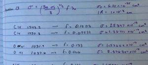
After a number of plots on my part and meetings with both my advisor and the man he met at the conference who gave him the idea, we had a plan. It turns out there have been observations of a galaxy where they were able to estimate the amount of absorption due to specific ions and elements – and from that they can estimate the density of these atoms. For this galaxy they found that there was very little nitrogen five (N V). One of the possible explanations for this is that there is some type of physics going on that is suppressing the amount of N V that is produced within the gas around the galaxy. I have access to simulations that looked at the influences of both hydrodynamics and conduction on this kind of gas (previous work done by my advisor) and I have code that can measure the amount of N V. So I looked at N V in these simulations and I saw that there was significantly less N V in the cases with conduction than without. This gave us the inspiration to try to match the simulations I have to the real data.

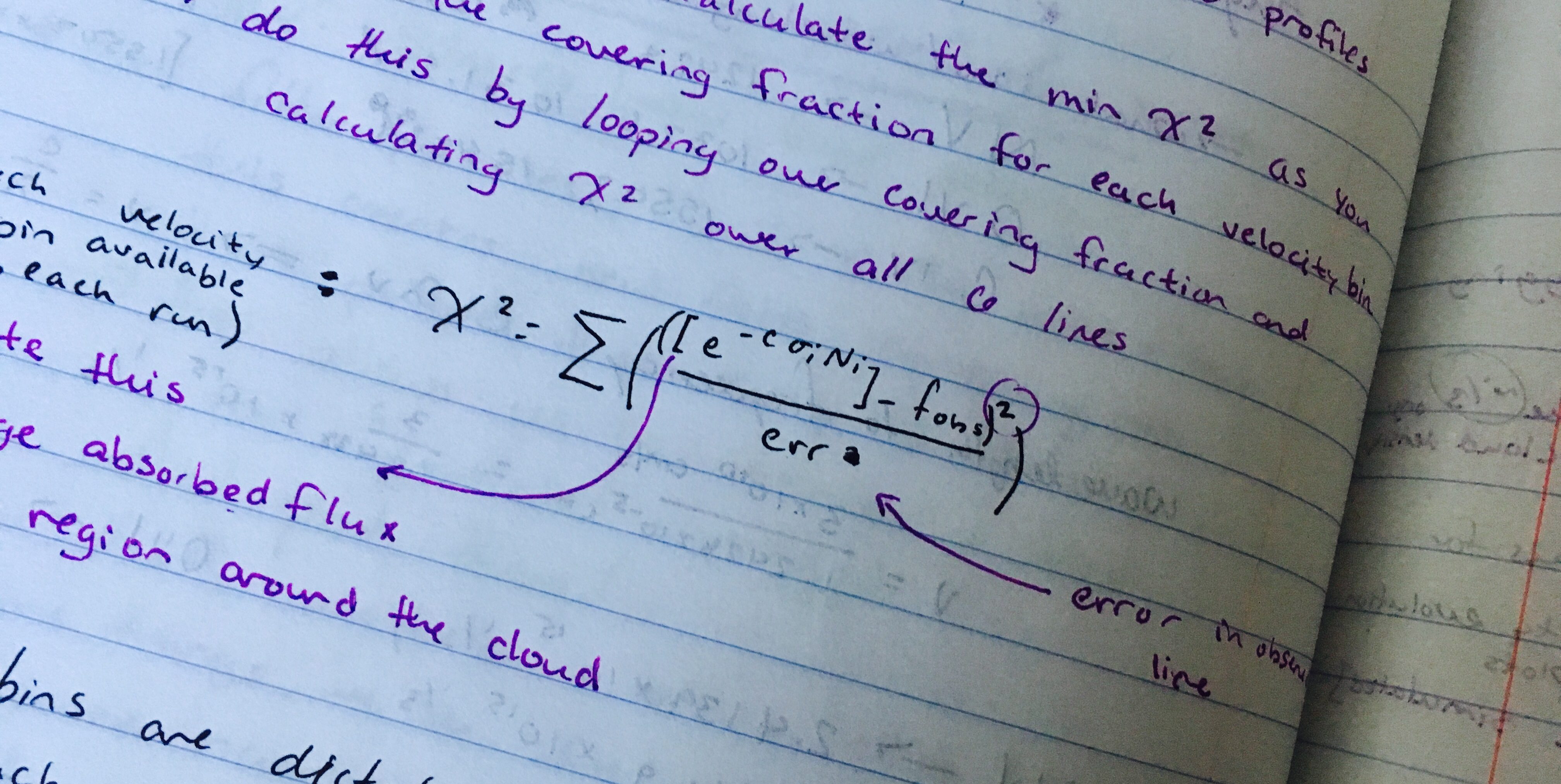
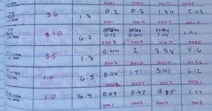
To do this I have created tables that allow my code to simulate the environment around this type of galaxy. I then used these tables to measure the density of various elements within the simulations. Finally – just this past week – I’ve been able to measure the average absorption we would expect if these simulations were actually observed out there in space. The hope for the next little while is to tweak this absorption to try to get it to fit the actual observation data. Some simulations I have might fit really well, some might fit horribly. This will then tell us what the environment is like around this observed galaxy, and what kinds of physics are apparent. If the conduction simulations fit well we know that conduction is significant within the gas around the galaxy. If they don’t fit, we know that conduction does not effect the gas very much.

However, what I am most excited about is that this kind of work is very easily extended. I can do the same kind of analysis, fitting the average absorption from simulations to observations, for many situations. I can do simulations with magnetic fields and look how the simulations fit. I can tweak simulations to include different types of winds and see if they fit observations better. This type of analysis can be applied to many different types of physics and many different observations of galaxies. In the words of my advisor, “If all that doesn’t make up a dissertation, then I don’t know what does.”